Rafa Santana

I am a physical oceanographer with expertise in the dynamics of coastal, sub- and mesoscale ocean variability from equatorial to polar regions (e.g., Santana et al.,2018, 2019 and 2021). My focus is to improve our understanding of variability in ocean conditions and how it impacts society using observations, numerical modelling, and data assimilation (e.g., Santana et al.,2020 and 2023). I work at the National Institute of Water and Atmospheric Research (NIWA), most specifically within the Coastal and Esturarine Group. At NIWA, my research targets at understanding past ocean conditions and future climate scenarios to see how these changes may affect society. An example of my work is shown in the video below, where the impact of waves generated by the Tropical Cyclone Harold was studied using SWAN wave model forced by winds from the Tropical Cyclone wind generator (TCwindgen) and the European Reanalysis 5 (ERA5).

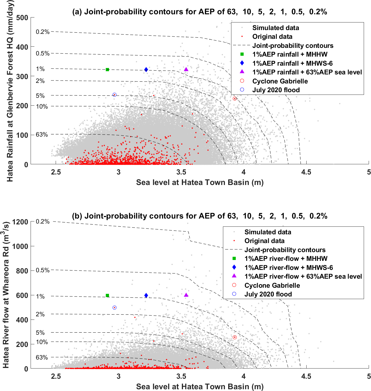
Left: maps of Significant Wave Height in metres (Hsig, rainbow shade and white arrows) and winds (black arrows) during Tropical Cyclone Harold. Right: timeseries at four different locations from the SWAN model forced by TCWindgen and ERA5.

east auckland current and cross shelf exchange

A year in the life of the East Auckland Current (EAuC)

In 2022, I graduated as a PhD in Marine Science and Mathematics at the University of Otago in conjunction with the National Institute of Water and Atmospheric Research (NIWA). My PhD focuses on understanding drivers of variability in the East Auckland Current (EAuC) and its impact on the shelf-slope connectivity and carbon export. The first chapter of my thesis is summarised in the article "Mesoscale and wind‑driven intra‑annual variability in the East Auckland Current" freely available at https://www.nature.com/articles/s41598-021-89222-3 . It tells about a year in the life of the EAuC. There, we study mesoscale eddies (ocean cylinders of aprox. 100 km diameter) that dominated the circulation for a total of 260 days and the EAuC which was present for 110 days. Winds played an import role by generating variability shorter than 30 days in the velocity and temperature.

Maps of Sea Surface Temperature (SST) spatial anomaly (coloured shade) (mean value in black), geostrophic (black arrows) and daily averaged in situ velocities (coloured arrows as in Fig. 1a) on (a) 11/5/2015, (b) 7/7/2015, (c) 26/8/2015, (d) 2/11/2015, (e) 6/1/2016, and (f) 18/4/2016 showing the mesoscale structures A1, C1, EAuC, A1, A2/C2, and C2, respectively.

Modelling the East Auckland Current

Surface and localised in situ observations are not enough to understand the full dynamics in the region. That's why we use numerical models that can provide daily 3D pictures of the oceans. In the figure below, we compare results from a model and observations from satellites and moored instruments. We can see that the model does a good job simulating the temperature structure. However, mesoscale eddy variability is not well represented.

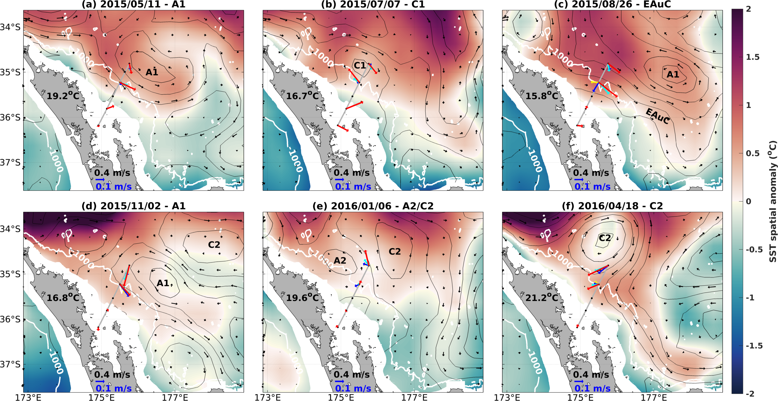
Figure caption: Left - Map of Sea Surface Height (SSH) (AVISO = black countors; Model = shade), geostrophic currents (AVISO = blue arrows; Model = black arrows), and in situ velocities (red, cyan, blue and yellow arrows). Right - Cross-section of temperature (In situ = coloured contours; Model = shade). The cross-section location is shown by the grey line on the map.

Data assimilation is needed

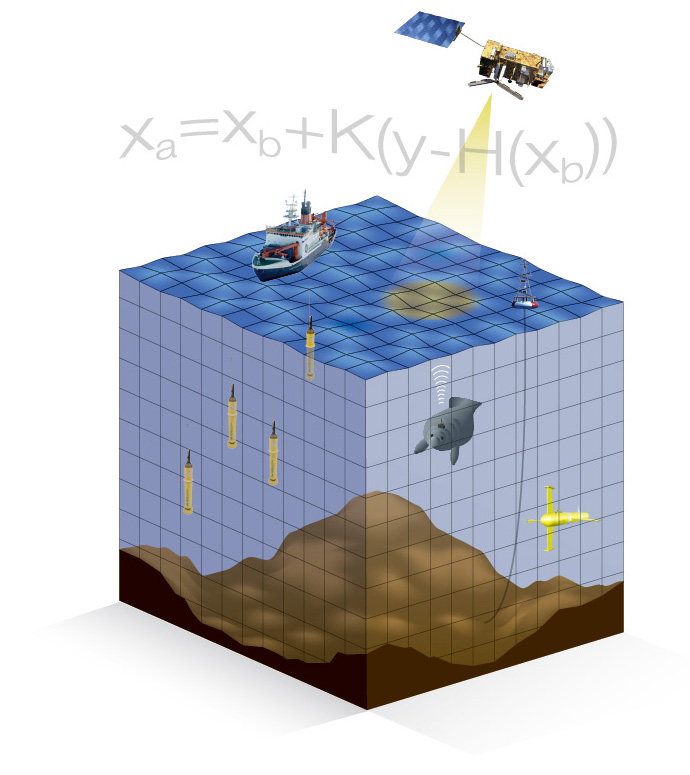
Mesoscale eddies are generated by instabilities which are unpredictable. Therefore, we need to incorporate satellite-derived and in situ data into the model to constrain its solution closer to observed values. This process is called data assimilation and aims to solve the equation below, which considers both model error and representativeness errors present in the observations (combined into K).

Figure source: Joint ECMWF/OceanPredict workshop on Advances in Ocean Data Assimilation.

Data Assimilation in the East Auckland Current

Remotely-sensed and in situ observations were assimilated into the model (ROMS) using 4D-VAR. Sea surface height (SSH) and temperature (SST) and mooring temperature, salinity, velocity from stations M3, M4, and M5 were assimilated. The setup and validation of these and other experiments are shown in Santana et al., (2023) . The video below shows that the simulation on the right (ASFUVTS-h or ASFUVTS-2days in Santana et al., 2023) better represents the mesoscale eddies in comparison to the freely evolving simulation on the left (Control-JRA55do).

Model comparison: freely evolving simulation (Control-JRA55d0 - left) model with data assimilation of SSH, SST, velocity, temperature and salinity from moorings (M3-M5). Variables compared are Sea Surface Height (AVISO = black countors; Model = shade), geostrophic currents (AVISO = blue arrows; Model = black arrows), and in situ velocities (red, cyan, blue and yellow arrows).

Eddy driven cross-shelf in the East Auckland Current system

Cross-shelf flows are ten times smaller than along shelf currents. Processes that promote cross-shelf exchange play an important role in renovation shelf waters and exporting material to the deep ocean. Here we used an eddy tracking algorithm to track eddies formed on the continental shelf (coastal eddies) to see their impact on generating cross-shelf exchange. We see that some eddies travel offshore while trapping river tracers (example: organic carbon) and may deposit in the deep ocean (video below).

Left: Map of river tracer (green shade) and coastal eddies' tracks (blue lines). Right: cross-section of river tracer (green shade) along the magenta line in the map.

Eddy-driven uplift on the continental shelfbreak

A space-time plot shows that cold-core (cyclonic) eddies can uplift cold waters onto the shelf causing negative temperature anomalies of -1.5oC, which might bring nutrient-rich waters onto the shelf and increase producticvity. These eddies might also play an important role in cooling down the shelf break during marine heat events, especially for expected future warmer climates.

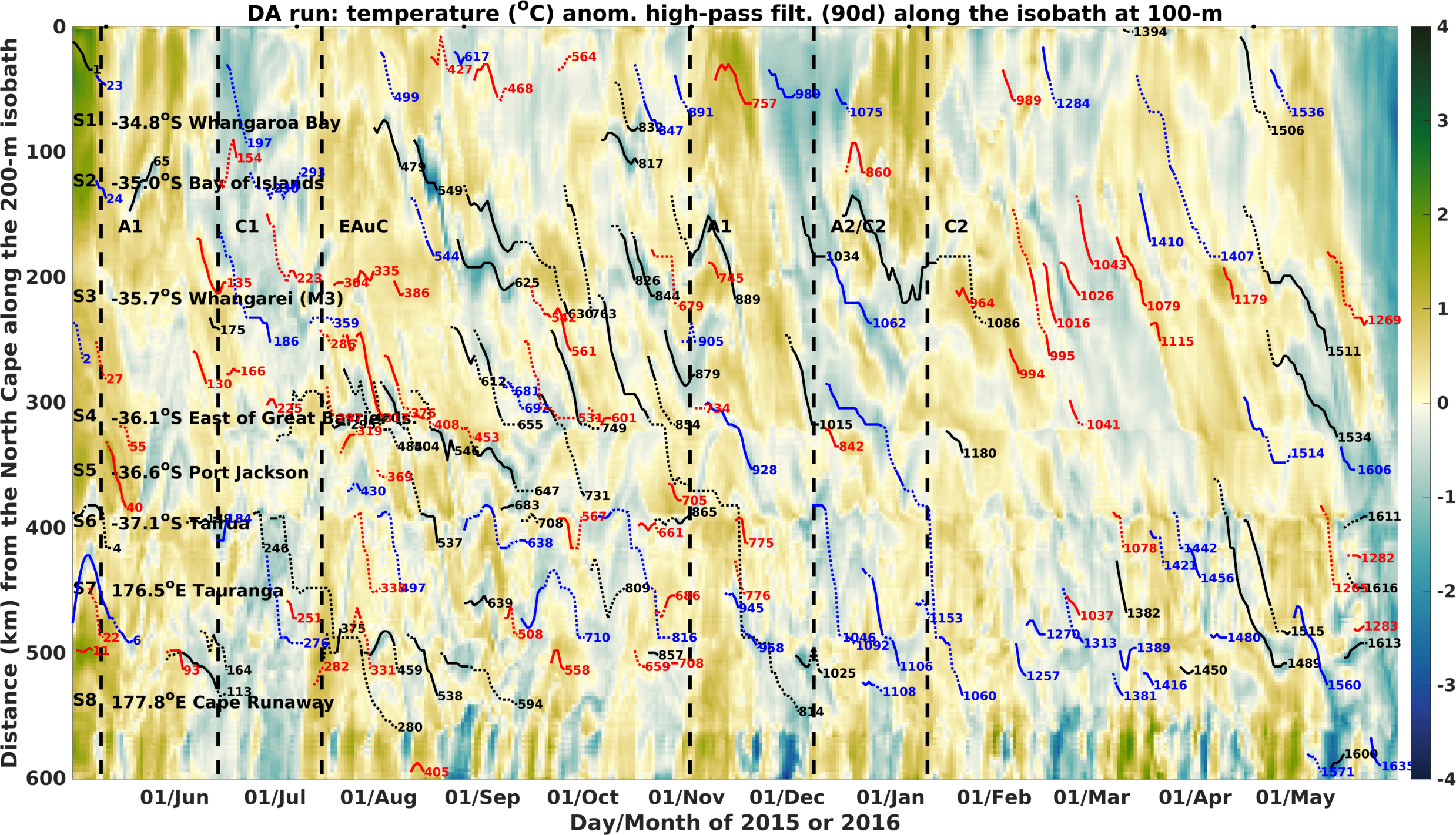Space-time plot of 100-m high-pass filtered (90 days) temperature time-anomaly along the 200-m isobath from DA run. Tracks of coastal (black) and slope (blue) cyclones, and anticyclones (red) that encroach (solid lines) onto the shelfbreak (200-m isobath) or translated away (dotted lines) from that isobath are shown. Location of the sections and neighbouring regions are shown along the y-axis. The acronyms A1, C1, EAuC, A1, A2/C2, and C2 represent the presence of mesoscale structures studied in Santana et al., (2021)

Polar science

I started to study polar regions as a research fellow at The University of Auckland, where I worked on the Scale-Aware Sea Ice Project (SASIP). I targeted at understanding ocean-ice interactions around Antarctica using the sea-ice model neXtSIM. An example of neXtSIM's application is shown in the video below (credit: Nansen Environmental and Remote Sensing Center).

Sea ice concentration in Fram Strait simulated by the Lagrangian sea ice model neXtSIM. Credit: Nansen Environmental and Remote Sensing Center.

Antarctic neXtSIM

My collaborators and I have implemented an Antartic version of neXtSIM which has been thoroughly validated (Santana et al., in prep.). We compare two versions of neXtSIM in this study using a modified Viscous-Elastic-Plastic (mEVP - used in climate models) and a Brittle Bigham-Maxwell rheology (science of material deformation). In the the mEVP run, sea ice moves slowly and fails to represent observed mesoscale drift features (video below). The BBM run improves the representation of sea ice ice at any given day compared to the mEVP rheology, and is able to reproduce cyclonic features in sea ice drift forced by atmospheric events. This happens because the BBM run reproduces ice fractures more realistically (previous video) which facilitates the transport of sea ice.

Daily Antarctic sea ice drift (km/h) from satellite observations (let), the modified Viscous-Elastic-Plastic (mEVP - centre) run, and the Brittle Bigham-Maxwell (right) run.